Measures of central tendency

Recommended: First read Measures of shape

A measure of central tendency (also referred to as measures of centre or central location) is a summary measure that attempts to describe a whole set of data with a single value that represents the middle or centre of its distribution.

There are three main measures of central tendency:

• mode
• median
• mean

Each of these measures describes a different indication of the typical or central value in the distribution.

The mode is the most commonly occurring value in a distribution.

Consider this dataset showing the retirement age of 11 people, in whole years:

54, 54, 54, 55, 56, 57, 57, 58, 58, 60, 60

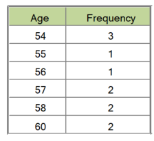
This table shows a simple frequency distribution of the retirement age data.

The most commonly occurring value is 54, therefore the mode of this distribution is 54 years.  

The mode has an advantage over the median and the mean as it can be found for both numerical and categorical (non-numerical) data.  

The are some limitations to using the mode. In some distributions, the mode may not reflect the centre of the distribution very well.  When the distribution of retirement age is ordered from lowest to highest value, it is easy to see that the centre of the distribution is 57 years, but the mode is lower, at 54 years.  

54, 54, 54, 55, 56, 57, 57, 58, 58, 60, 60

It is also possible for there to be more than one mode for the same distribution of data, (bi-modal, or multi-modal).  The presence of more than one mode can limit the ability of the mode in describing the centre or typical value of the distribution because a single value to describe the centre cannot be identified.

In some cases, particularly where the data are continuous, the distribution may have no mode at all (i.e.  if all values are different).

In cases such as these, it may be better to consider using the median or mean or group the data into appropriate intervals and find the modal class.  

The median is the middle value in distribution when the values are arranged in ascending or descending order.

The median divides the distribution in half (there are 50% of observations on either side of the median value). In a distribution with an odd number of observations, the median value is the middle value.  

Looking at the retirement age distribution (which has 11 observations), the median is the middle value, which is 57 years:  

54, 54, 54, 55, 56, 57, 57, 58, 58, 60, 60 

When the distribution has an even number of observations, the median value is the mean of the two middle values.  In the following distribution, the two middle values are 56 and 57, therefore the median equals 56.5 years: 

52, 54, 54, 54, 55, 56, 57, 57, 58, 58, 60, 60

The median is less affected by outliers and skewed data than the mean and is usually the preferred measure of central tendency when the distribution is not symmetrical.  

The median cannot be identified for categorical nominal data, as it cannot be logically ordered.

The mean is the sum of the value of each observation in a dataset divided by the number of observations. This is also known as the arithmetic average. 

Looking at the retirement age distribution again: 

54, 54, 54, 55, 56, 57, 57, 58, 58, 60, 60

The mean is calculated by adding together all the values (54+54+54+55+56+57+57+58+58+60+60 = 623) and dividing by the number of observations (11) which equals 56.6 years.

The mean can be used for both continuous and discrete numeric data.

The mean cannot be calculated for categorical data, as the values cannot be summed.

As the mean includes every value in the distribution the mean is influenced by outliers and skewed distributions.

The population mean is indicated by the Greek symbol µ (pronounced ‘mu’).   When the mean is calculated on a distribution from a sample it is indicated by the symbol x̅  (pronounced X-bar). 

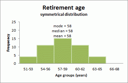
When a distribution is symmetrical, the mode, median and mean are all in the middle of the distribution.  The following graph shows a larger retirement age dataset with a distribution which is symmetrical.  The mode, median and mean all equal 58 years.

When a distribution is skewed the mode remains the most commonly occurring value, the median remains the middle value in the distribution, but the mean is generally ‘pulled’ in the direction of the tails.  In a skewed distribution, the median is often a preferred measure of central tendency, as the mean is not usually in the middle of the distribution.  

A distribution is said to be positively or right skewed when the tail on the right side of the distribution is longer than the left side. In a positively skewed distribution it is common for the mean to be ‘pulled’ toward the right tail of the distribution.  Although there are exceptions to this rule, generally, most of the values, including the median value, tend to be less than the mean value.  

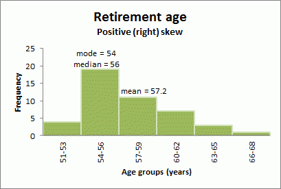
The following graph shows a larger retirement age data set with a distribution which is right skewed.  The data has been grouped into classes, as the variable being measured (retirement age) is continuous.  The mode is 54 years, the modal class is 54-56 years, the median is 56 years, and the mean is 57.2 years.

A distribution is said to be negatively or left skewed when the tail on the left side of the distribution is longer than the right side. In a negatively skewed distribution, it is common for the mean to be ‘pulled’ toward the left tail of the distribution.   Although there are exceptions to this rule, generally, most of the values, including the median value, tend to be greater than the mean value. 

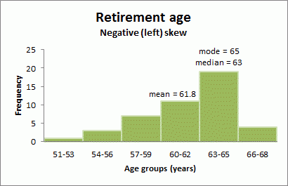
The following graph shows a larger retirement age dataset with a distribution which left skewed.  The mode is 65 years, the modal class is 63-65 years, the median is 63 years and the mean is 61.8 years.

Outliers are extreme, or atypical data value(s) that are notably different from the rest of the data.

It is important to detect outliers within a distribution, because they can alter the results of the data analysis.  The mean is more sensitive to the existence of outliers than the median or mode.  

Consider the initial retirement age dataset again, with one difference; the last observation of 60 years has been replaced with a retirement age of 81 years.  This value is much higher than the other values, and could be considered an outlier.  However, it has not changed the middle of the distribution, and therefore the median value is still 57 years.  

54, 54, 54, 55, 56, 57, 57, 58, 58, 60, 81

As the all values are included in the calculation of the mean, the outlier will influence the mean value.    

(54+54+54+55+56+57+57+58+58+60+81 = 644), divided by 11 = 58.5 years

In this distribution the outlier value has increased the mean value.  

Despite the existence of outliers in a distribution, the mean can still be an appropriate measure of central tendency, especially if the rest of the data is normally distributed.  If the outlier is confirmed as a valid extreme value, it should not be removed from the dataset. Several common regression techniques can help reduce the influence of outliers on the mean value.

External links:
easycalculation.com - Mean, Median, Mode Calculator
calculatorsoup.com - Descriptive Statistics calculator
calculatorsoup.com - Mean Median Mode calculator