Recent applications of supermarket scanner data in the National Accounts

The Australian Bureau of Statistics (ABS) has been collecting ‘point of sale’ systems data from supermarkets, otherwise known as scanner data, since 2011. The main use of scanner data in the ABS to date has been in the compilation of the Consumer Price Index (CPI). Scanner data has enormous potential for use in official statistics due to its coverage, frequency and granularity; however, to date there has been limited work to develop methods using this data to compile National Accounts.

This paper presents recent ABS work using supermarket scanner data to inform food consumption by households. The paper details how supermarket scanner data can be used to produce high quality indicators of household food consumption in both current price and volume terms. Additionally, the paper describes how scanner data can provide additional insights into changes in household food consumption patterns as well as further plans for development in the National Accounts.

Authors: Andy Peisker, Tom Lay and Michael Smedes

National Accounts, Macroeconomic Statistics Division

Collecting data from ‘point of sale’ systems of businesses and government organisations is becoming increasingly common in Australia and around the world. A good example is ‘scanner’ data collected in supermarkets. These datasets offer enormous benefits for National Statistical Offices (NSO’s) due to their high frequency, coverage and granularity. They have the potential to reduce substantially collection costs and the reporting burden placed on the community. The ABS is increasing our use of these statistics.

Since 2011 the ABS has been receiving “scanner data” from major supermarket chains in Australia. This data has been used extensively in the calculation of the Consumer Price Index (CPI) and now contributes approximately 16% to its compilation.¹ The richness of the scanner data means it has a number of other statistical applications, including in the compilation of Household Final Consumption Expenditure (HFCE) in the National Accounts. To date, there has been limited application by NSO’s. This paper highlights recent ABS work using scanner data in the Australian National Accounts, specifically for HFCE Food estimates. The paper also outlines ABS plans to expand the use of this dataset within the compilation of the National Accounts including some future projects on integrating scanner data into household consumption measurement.

The ABS currently receives data from major supermarket chains, this data accounts for approximately 84% of all expenditure through supermarkets. The data are essentially a “census” of sales for these chains, and are supplied weekly with the following dimensions:

• Product/item description
• Quantity of items sold
• Dollar value of items sold
• Geographical location

The primary driver for acquiring this data was for enhancing the CPI, in terms of reducing collection costs in supermarkets, reducing collection errors and increasing coverage of collected prices. Scanner data has also led to the development of multilateral indexes which are more responsive to product substitution over time, and less vulnerable to large shifts in consumer behaviour.²

Household consumption, (formally referred to as Household Final Consumption Expenditure in the National Accounts) measures the value of goods and services purchased by Australian households and specifically excludes those purchased for business purposes. It is the largest component of Gross Domestic Product (GDP) accounting for around 60% and a major contributor to the Household Saving ratio. The ABS publish both annual and quarterly estimates of household consumption and these are broken down using the Classification of Individual Consumption by Purpose (COICOP) and by State and Territory.

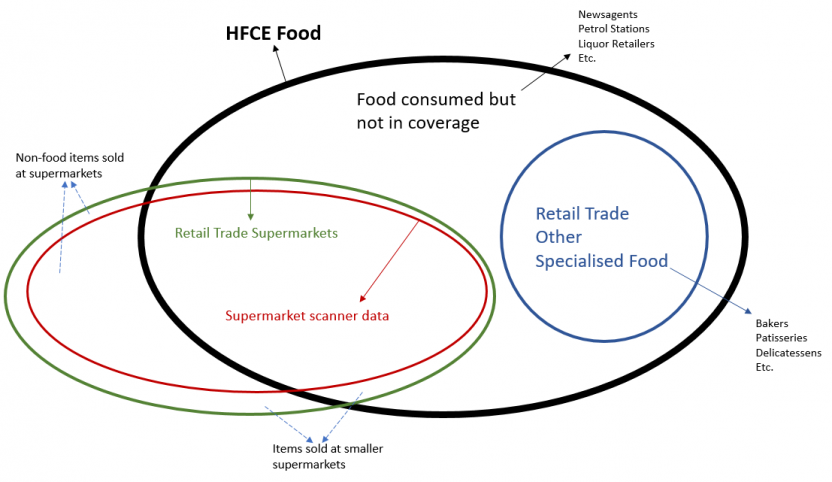
Nearly 80% of food consumed by households in Australia is purchased through Supermarkets. Therefore, scanner data is most relevant in the compilation of the “Food” category within household consumption. This category includes all food and non-alcoholic beverage products purchased by households that have not been pre-prepared as a catering service. It excludes any food consumed in restaurants, pubs, bars, hotels, but includes almost all food products purchased at supermarkets (see Figure 1). In total the Food consumption category constitutes approximately 10% of household consumption, and around 6% of GDP.³

Household consumption estimates are currently compiled by utilising the Household Expenditure Survey (HES) and the Retail and Wholesale Industry Survey (RIS/WIS) to build up “benchmark” levels of HFCE by COICOP. Both the HES and RIS/WIS are infrequent data sources and are not available every year. For years where these sources are not available, the monthly ABS Retail Trade Business survey is used as an “indicator” which is applied to the benchmarks to produce annual and quarterly estimates.  

There are limitations to the Retail Trade Survey as an indicator of household food consumption. The most notable is it is an industry-based survey and does not collect any information about the products sold. For example, estimates for “Food retailing” are used as the indicator for household consumption of food, although this will include non-food sales in food retailers such as supermarkets. Information from the RIS/WIS is used to determine the composition of food and non-food products sold and this composition is held fixed between survey cycles. It is also assumed that household expenditure on food and non-food products grows at the same rate each quarter. Supermarket scanner data can be used to overcome these limitations and potentially improve the accuracy of household consumption estimates.

There has been limited use of scanner data in the Australian National Accounts with scanner data currently only used as a direct input to compile the Cigarettes and Tobacco” category of household consumption. As an initial step to widening the use of this dataset, the ABS has produced experimental quarterly indicators of household consumption of food using the supermarket scanner data.

At this stage, these estimates have been produced:

• In original terms only (no seasonal adjusted or trend estimates)
• For both Current Price Values and Chain Volume Measures
• At the Australia and State & Territories levels

Selected results from the experimental work are presented in figures 2 to 5. These have been presented alongside existing estimates of Retail Trade and HFCE to illustrate how they compare over time. There are some differences in movements mainly due to scope and coverage. However, the experimental estimates tell a similar story around the patterns of food consumption.

The high frequency and granularity of the scanner data present opportunities to produce additional insights into changes in household consumption in a way which existing data sources don’t. This has been of enormous value, particularly, in the last 12 months as the economy has been impacted by natural disasters and the COVID-19 pandemic.

The geographical dimension of the scanner data means estimates below the State level can be produced. This has enabled the ABS to analyse changes in food spending in metropolitan and regional areas. In March 2020 quarter, parts of Australia were impacted by bushfires. Tourism related activity such as domestic travel, accommodation and food services declined in the affected areas. The fall in the number of people visiting regional areas and supply chain disruptions due to the bushfires, are evident in the scanner data for food in regional areas.

Food sales were stronger in capital cities than they were in regional areas across all of the states and territories, particularly New South Wales and Victoria (Figure 6).

Scanner data also provides the ability to examine the drivers in food consumption by analysing at product level sales. The onset of the COVID-19 pandemic and subsequent lockdowns and restrictions introduced by Governments, led to shifts in household consumption behavior. There was a significant increase in spending on food items at supermarkets as households prepared for an extended period at home. Analysis of detailed product data (figure 7) shows that this behavior was most evident in “other cereal products” which includes cereals, pastas, rice and flour.

In the Australian National Accounts, key economic variables such as HFCE are produced for both “current price values” (CPVs) and “chain volume measures” (referred to as “volumes” or CVMs). CPVs are derived by aggregating dollar values for any given time period. Changes in CPVs over time will include the effects of inflation. CVMs remove inflation effects by applying a technique called “deflation” using an appropriate price index such as the CPI.

The CPI is a measure of pure price changes. This means the CPI should ignore price changes that result from variations in the quantity or quality of items. In reality, the quality and quantity of items in the basket can vary and new products can be introduced. For example, a jar of sauce can become smaller in weight, or the quality of a computer can improve if it has more processing speed.

The ABS tries to remove any price changes that result from changes in quality or the mix of items that households buy. Following the previous examples, the ABS would calculate the price of the sauce assuming that the weight remained the same and compare it with the price in the previous quarter.⁴

When quality adjusted price indexes such as CPI are used to deflate CPV measures, the derived volume measures will encompass changes in both the quantity and quality of expenditure of the product. The relationship between CPV and CVM’s can be represented as follows:

Consider the product category of "Bread". Suppose that the general price of bread increases 10% between quarter 1 (Q1) and quarter 2 (Q2).

In Q1, a consumer purchased one loaf of supermarket brand multigrain bread (500g) which costs $2.50. In response to the rising price of bread, the consumer switches to purchasing one loaf of supermarket brand white bread (600g) which costs $2.25 in Q2.

The volume index is derived as the ratio of current price expenditure and price index change. The quality index is derived as the ratio of the volume index and the quantity index.

Assuming all else stays constant, there is a decline in volumes of 18.2%, which on face value could be taken to indicate that consumers reduced their consumption of bread in response to rising prices. However, further disaggregation of volumes show that the quantity of bread (in grams) increases 20% between Q1 and Q2. The quality of bread expenditure has reduced by 31.8% indicating that the bread purchased in Q2 has around one third less "utility" per kilogram consumed.

The estimates for volume, quantity and quality (Figure 8) show that over time, quantities of food consumed by households tend to remain relatively stable over time. Changes in quality appear to drive most of the changes in overall volumes of consumption. This is particularly apparent in the period from June 2019 to March 2020, where consumers reduced the quality of food purchases. Changes in quality tend to be inversely related with changes in food prices (Figure 9). That is, in times of rising prices, consumers will tend to reduce the quality of the food they consume. This substitution behavior is noticeable in the period from June 2019 to March 2020 which saw elevated levels of food price inflation as a result of the drought.  In a real-world sense, this might include shifting expenditure to cheaper brands of food products, or cheaper varieties of fresh foods such as meat, fruit and vegetables.

This analysis also extends to better understanding of volume movements following the onset of COVID-19. In June quarter 2020, volumes of food consumption returned to more normal levels following significant stockpiling activity by households in March. As dine-in services at cafes and restaurants were closed down to help manage the pandemic, scanner data showed that households increased the quality of their food expenditure (e.g. higher quality ingredients), presumably in response to the closure of dine-in services at cafes and restaurants and more time cooking at home.

The granularity of the scanner data allows for additional analysis to determine which products are driving this behavior. Figures 10, 11 and 12 show some of the products which have seen larger price rises over 2018-19. There is a clear inverse relationship between movements in price and quality, with consumers reducing quality, but maintaining quantity, in response to rising prices. The opposite is also true such that when inflation is low or falling, consumers will tend to increase the quality of their purchases and maintain quantity.

The analysis and applications presented in this paper represent only a small part of the enormous potential for scanner data use in the National Accounts and ABS more broadly. The ABS is looking to build on this current work and extend its use of this dataset in the National Accounts.

• Develop experimental estimates of Food HFCE using scanner data. The ABS will develop benchmark (Level) estimates of HFCE Food using scanner data.  This will allow for estimates to be built up from low-level product data and be mapped to the Input Output Product Classification (IOPC) which is considered the building block of HFCE. These estimates would be experimental for a period to allow the ABS to assess its performance against existing estimates before considering them to replace existing sources. Work is being undertaken to develop methods and techniques to overcome the scope and coverage issues which exist in the scanner data. These include accounting for food purchases outside supermarkets, removing non-resident and business expenditure, and accounting for supermarkets which do not provide data to the ABS.
• Improve accuracy of quarterly indicators. Under the current approach of using the Retail Trade Survey as a quarterly indicator of HFCE Food, the composition of food and non-food sales in supermarkets is assumed to be a fixed ratio. Due to the lack of timely product information, this ratio derived from the 2012-13 RIS/WIS. Using the product detail in the scanner data it is possible to derive estimates which provide an indication of movements in sales of food and non-food items. These estimates are useful in their own right but could also be used to improve the accuracy of existing estimates of HFCE food by better accounting for disparate movements in expenditure on food and non-food items.
• Produce additional insights on household consumption. While there have already been some insights produced previously by the ABS using the scanner data, there is potential for further insights. These include further geographic disaggregation to Statistical Area Level 4 (SA4) along with more detailed drivers at the product level. These will be shared through ABS analytical pieces such as spotlights and commentary.  

The method for producing quarterly volume indicators from the scanner data consists of four steps, described below.

Step 1 – Data preparation and filtering for quarterly analysis

The ABS receive weekly revenue and quantity aggregates from supermarkets, therefore quarterly volume analysis requires some pre-aggregation from weekly to quarterly revenues. Where a week is divided across two quarters, any revenue is assumed to be split proportionally according to the number of days in each of the two quarters. As the volume analysis relates to food consumption, all non-food is identified based on the product’s expenditure class (EC), and removed if the product EC is not a food EC, or if the EC field is missing. The EC is assigned to the products in an automated way using the ABS Intelligent Coder, which classifies the products by interpreting according to the text descriptions provided by the supermarkets.

Scanner data sales are from the perspective of the supermarkets, rather than from households. As part of this analysis, there is no attempt to filter out sales to non-household entities such as businesses (e.g. restaurants/cafes), as information about the customer type is not collected by the supermarkets at the point of sale. However, as the focus of the analysis is on household consumption indicators (i.e. movements) rather than levels, this is not seen as a major issue and the assumption is made that business sales as a proportion of the total remain stable over time.

Step 2 – Produce quarterly current price estimates

Current price and movement indicators were produced from the quarterly revenue files produced in Step 1, which assumes that supermarket sales are predominantly to households. For the current analysis, more interest was placed in movements, as pseudo-levels (raw aggregates of revenue) could be affected by imperfections such as sales to businesses, as well as the rates of coding to expenditure class (e.g. food products not being correctly classified and being excluded from levels). Level imperfections in the pseudo-levels were not seen as a quality risk to movement estimates as the coding success rates tended not to change greatly between consecutive quarters. The movements were generated by aggregating quarterly revenue to the relevant dimension (Geography and EC) and taking the percentage change in the pseudo-levels.

Due to the relatively short time span over which fit-for-purpose scanner data exists seasonally adjusted estimates are not produced a part of this analysis. This reflects standard ABS practices that recommend at least 6 years for quality assuring seasonal adjustment quality. Instead through the year original estimates are presented and are a good means of accounting for seasonal influences in growth.

Step 3 – Produce Supermarket Price Index (SPI)

Volume analysis requires a price index, which for this analysis was compiled from the scanner data rather than relying on published indexes such as the CPI. This enables the production of price indexes which are more consistent with the scope of the current price supermarket sales being deflated. Comparisons indicate that at the total food level, the CPI and SPI had very similar movements over time, however the differences were observable at the volume level.

The method used to produce the “supermarket price index” (SPI) was the multilateral index method, introduced into the ABS in 2017, and which is now an established method in the production of CPI for certain expenditure classes. The SPI were produced at the EC, state and national total levels. It is possible to produce SPI at lower levels, which would facilitate chained volume aggregation to higher levels via product-level quantity and price series, this was seen as marginal benefit for substantially larger effort. To facilitate direct volume compilation, SPI are only produced for the levels at which volumes would be analysed which are EC, state and national.

Step 4 – Produce volume estimates

Volume growth is measured “directly”, by dividing the CPV movements by SPI movements at the same aggregation level as the desired volume, rather than at lower levels and aggregating through chain-linked index methods used to compile CVM’s in economic statistics including the National Accounts. This is seen as a fit-for-purpose approximation due to the nature of the economic concepts and their relative stability over time, for which this approximation should yield little difference from the much more effort intensive “exact” CVM approach. The exact approach is beneficial where large compositional shifts can cause significant differences between the price index and the IPD, resulting in measurement errors.

This produces volumes time series at the level of expenditure class, state and national total. As with all chain volume measures published in ABS economic statistics, movements are not additive between the states / ECs and the national total, though the residual should typically be small given the composition of consumer baskets is relatively stable over time.

1. Web scraping in the Australian CPI

2. Information Paper: Making Greater Use of Transactions Data to compile the Consumer Price Index, Australia, 2016 
3. Based on 2019-20 expenditure at current prices 
4. Note that the definition of quality in the CPI is slightly different to the concept of quality defined in this analysis. The CPI concept encompasses all changes in volumes for any given product.  
5. See for example the discussion of consumer theory in Varian, H. Intermediate Microeconomics, 9th Edition. New York: W.W. Norton, 2014