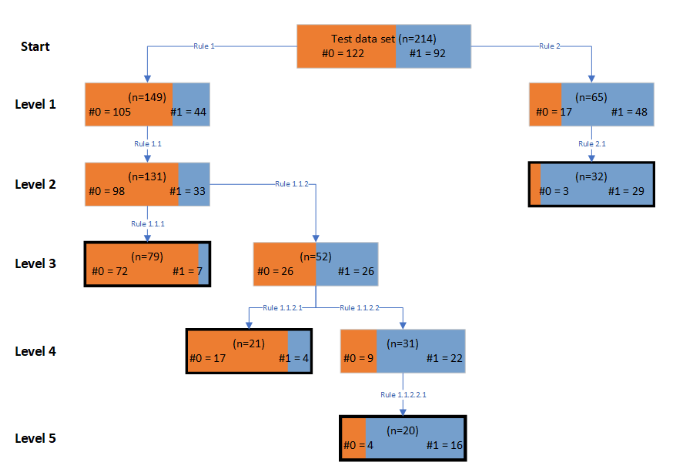
Producing Official Statistics from Linked Data — Technical Report

This project investigated one thread of the general proposition that Australian Bureau of Statistics’ Business Characteristics Survey (BCS) data could relate to outcomes for individual businesses. This investigation used BCS data for financial years (FY) 2015-16 to 2019-20.  

Owing to what seemed a relatively direct relationship between a BCS data item and an outcome, we used compprof_bcs to consider relative profitability of 1070 “in-scope” businesses over the three FY 2017-18 to 2019-20. Profitability values permit the assignment of each business to either a “high profitability score” group, or a “lower profitability score” group. This casts the investigation as a binary classification problem, followed by an interrogation of how classifications were made. The existence of any features having certain values for only one group of businesses (that is, features with a high “feature importance”, FI) indicates a systematic difference between groups. 

Random forests were used for classification. Given the dataset features, “raw” FIs were determined using the “permutation” method. Individual trees in a random forest can produce different raw FI values for a given feature. Hence, we calculated the mean and standard deviation of raw FIs associated with individual features. To aid interpretability, raw FIs for all features were used to produce “normalised” mean FIs that sum to 1.  

The dataset contained several highly correlated features, which can distort results. Accordingly, a systematic process was used to remove such features. Features were also removed following the calculation of normalised FIs if their 95% confidence interval was not completely above zero. The random forest was then refit to the reduced training set. 

Following some rounds of this process, we arrived at a reduced dataset of 17 features. A random forest classifier applied to a training set and test set obtained from this reduced dataset showed adequate performance (classification accuracies of approximately 82% and 79% respectively) in each case.  

Proceeding to an inspection of FIs showed that the five largest mean normalised FIs (signalling the most influential features) relate to two different “relative change” features for time points in the last three years of the dataset. Placed in decreasing order, compprod_bcs (“Productivity”) are the first, fourth, and fifth entries. The second and third-largest entries relate to compsogs_bcs (“Income from the sales of goods or services”).  Most of the remaining features have far smaller mean normalised FIs, indicating a smaller influence on classifier performance. However, these may still make some contribution to understanding how classification occurs, and feature in the decision rules that conclude the report.

This technical report accompanies the summary of outcomes of a project that investigated one thread of the general proposition that Business Characteristics Survey (BCS) data can relate to business outcomes¹​. We have specifically used BCS data (accessible through BLADE² ) to investigate the relationship between BCS variables (or “features”) and a derived quantity relating to business profitability. We propose that a machine learning (ML) classifier can recognise those features of BCS data that contribute to a business being regarded as either in a “high profitability score” group, or a distinct “lower profitability score” group. 

Our proposed groupings inform the “labels” for businesses in our classification problem. We form these labels with reference to the BCS variable “compprof_bcs”. This variable holds the assessment of each business of their current year’s profit relative to the previous year’s. Aside from certain troublesome values (causing the removal of some businesses from the dataset), valid responses are that profit has 1. decreased, 2. stayed the same, 3. increased. 

Initial investigations considered the performance of various classifiers, and approaches to preparing data for use with these. The task for each “pipeline” combining data processing and a classifier was to train the classifier on part of the (appropriately processed) data (the training set), reserving a portion of the data for testing (the test set, not seen in training). A standard way to judge a pipeline’s value is to consider the “classification accuracy” it can produce. We can validate predictions and compute classification accuracy here as we can compare labels predicted by the classifier with the true labels across all businesses considered. More specifically, we determine whether a pipeline that showed acceptable accuracy in classifying training-set instances can also produce an acceptable classification accuracy for the test set.  We may consider a classifier to be useful if its accuracy can substantially outperform naïve methods similarly applied to the data. 

Given the aim of the project and time constraints, attention was confined to classifiers able to directly produce “feature importances” (FIs): a measure of the influence individual features have on the classification. Following the time available for experimentation, a random forest classifier showed the best test-set accuracy. As this result was considered acceptable, we could proceed to interrogate the FIs. 

The remainder of this document is organised as follows. Section 2 provides an overview of the processing steps applied to BCS data that yielded the dataset considered in this study. Limitations of the data are also noted. Section 3 provides an overview of classification results obtained with a baseline method, and a brief description of the use of a random forest classifier and associated results. Section 4 presents the FI that result from the trained random forest classifier found in Section 3. The body of the paper concludes with some discussion of results in Section 5.  

Appendix A summarises the data processing used to replace missing values in certain features where these are a consequence of the path of a respondent through the survey. In such cases, a negative response to one question permits us to replace a missing value code in data items for related questions with a negative response. This type of process has substantially reduced the amount of missingness in some features, and either reduced the amount of infilling necessary, or led to features being retained that would otherwise have been excluded due to an unacceptably large number of missing values.

BCS data has many variables that are common to each of the financial years (FYs) 2015-16 to 2019-20, making this a suitable period for investigation. 

The in-scope population of businesses in the BCS data are those which: 

1. Have their identifier (BCS feature “id”) appear in data for each of the FYs from 2015-16 to 2019-20. 
2. Have compprof_bcs for each of the FYs 2017-18, 2018-19, and 2019-20 taking an informative value (i.e. in the range from one to three inclusive). 

These conditions led to an in-scope dataset of 1070 businesses. 

The decision to use BCS data over the selected five-year period was informed by preliminary inspection. This prompted us to make certain decisions about which features to include in the study dataset. Selecting features that are available for each year of the chosen dataset (that is, not missing for every business in the in-scope sample due to BCS changes) avoids systematic missingness and permits the study to be framed as a time-series classification problem. However, many BCS features are not present in all FY of the dataset.  

It was decided to limit the data range to the FYs 2015-16 to 2019-20³ ⁴ ⁵ ⁶ ⁷ so that a substantial number of features were potentially available for exploratory analysis. A substantial number of features appearing during this time were available for the entire dataset. However, it was decided to retain some variables which were not available only for the 2019-20 FY to broaden the features considered.   

Following these choices, it was decided to retain only those variables which had less than 20% of values missing. This cutoff was applied with reference to whether a feature was available for only four years, or for all five years in the BCS data. (See Section 2.2 for more on how systematic missingness was treated before we applied this judgement.) The exceptions were: 

1. id (this was required for all business in the in-scope dataset), 
2. compprof_bcs (see the discussion of labels above). 

The result was an in-scope dataset of 154 features with 119 being available over the five FY, and 35 systematically missing from the 2019-20 data. Not included in these features are “id” and the FY (which serve as indices in the dataset), and compprof_bcs used to produce our labels. 

There are two particular cases where infilling of missing values is necessary. In the first case, BCS data has various instances where a specific reason causes a BCS feature to have a substantial number of missing values. In such cases, we can use the logic of the BCS to confidently replace a missing value with another value that is logically consistent with the respondent’s other answers. This has substantially reduced the missingness for various features, permitting the retention of many that would otherwise be omitted. The specific processes used to address missingness for certain features are described in Appendix A. 

The second case where infilling is required is when data is “missing at random”.  Of the 154 features retained, 138 are categorical (possibly ordinal) and typically take values from a small range of integers (examples of “low-cardinality features”). Missing values for such a feature at a given time point were replaced by the mode of the feature at that time point. The remaining 18 features (examples include busopyr_bcs and busownyr_bcs, empoth_bcs, empprop_bcs, empsaldr_bcs, and emptotal_bcs) are numerical, and have a larger range (“high-cardinality features”). Aside from busopyr_bcs (business years of operation, regardless of ownership) and busownyr_bcs (number of years operating under current ownership) which were handled separately, missing values in a numerical feature at a given timepoint were replaced by the median of that feature at that time point.  

To obtain the label for a business in the in-scope population, their most recent three years (that is, from FYs 2017-18, 2018-19, and 2019-20) of compprof_bcs values were summed to yield an overall “profitability” score. Recall from the introduction that useful compprof_bcs values for this study are: 1 (decreased), 2 (stayed the same), and 3 (increased). As such, the profitability score can range from three to nine. The distribution of scores across the in-scope business population is shown in Figure 1. 

To aid classification, it is appropriate to avoid: 

• subdividing the dataset too finely (creating many potential categories, where some have few instances), and  
• producing categories of very different sizes (“unbalanced” classes).  

Mindful of these points, we used the profitability score to divide businesses into two categories of similar sizes. A business having a score in the range 7-9 defines that business as belonging to the “higher profit score” category (label "1” for implementation). Alternatively, a score in the range 3-6 assigns a business to the “lower profit score” category (label “0”). 

Following this assignment, 461 businesses have label 1, and 609 businesses have label 0. 

The intent of using an aggregate score is that it permits the formation of categories able to capture general trends in business profitability. That is, the total can allow a business to have one particularly good (or bad) year on the compprof_bcs scale, and still be included in the lower (or higher) score category due to its overall performance.  

We can demonstrate how the scoring system allows for some variability in performance by considering the membership of the higher-score category in detail. The category is comprised of businesses with reported profitability resulting in: 

• score 9: profit increased for each of the three years, 
• score 8: profit increased for two years in the range and unchanged profit for one year, 
• score 7: profit increased for two years and decreased for one year, or, profit increased for one year and unchanged for two years. 

Notably the component with a score of seven may admit businesses with an unprofitable year to the category. We can justify this possibility through a thought experiment considering businesses with a strong commitment to matters like workforce training, innovation or diversifying its markets. We would expect such commitment to support profitability over time. However, such businesses could still have a decrease in profitability in one isolated year due to a generally unfavourable business climate that year. As such, we choose to include such a business in the high-score category, rather than include it in a category of businesses which have a profit decrease more regularly. 

An extension of the above argument is that businesses with a generally low profitability should not be confused with other businesses due to one uncharacteristically good year. In a similar manner to the above, consider the lower-score category, composed of businesses with profitability reported with the result: 

• score 6: three years of unchanged profitability, or, one year each of unchanged, increased, and decreased profitability, 
• score 5: one year of decreased profitability and two years unchanged, or, two years of decreased profitability and one year of increase,   
• score 4: two years of decreased profitability, one year unchanged, 
• score 3: three years of decreased profitability. 

As before, there is some variability in this category as the components with a score of five or six can admit businesses that have one profit increase to the group. However, such businesses do not share the characteristic of higher-score businesses of having more profit increases than decreases. 

This study was subject to certain limitations which are outlined in the next subsection. 

This pilot study was subject to certain constraints, such as the time available, and was limited to BCS data. Other constraints followed from the nature of the choices made or the data itself. We shall document some study limitations below, expecting that this may be useful for any further work.  

2.4.1 In-scope dataset

Recall Section 2.1’s discussion of how the in-scope dataset was defined. Conditions A and B employed there led to the exclusion of certain businesses from the dataset. We shall consider these exclusions, and any consequences, below.  

Condition A acts to exclude businesses from the in-scope dataset that are not present in the BCS data for each FY from 2015-16 to 2019-20. As such, we have systematically excluded any business which: 

• ceases trading in any year of the study range, or, 
• commences trading after the 2015-16 FY but not after 2019-20 FY. 

These conditions are potentially significant to this study. Consider the first condition. Suppose that some businesses were wound up at some point during the FYs from 2015-16 to 2019-20 due to being inadequately profitable. (That is, such businesses have outcomes similar to those of our lower profit score group.) Further suppose that such businesses had certain characteristic features. Then, the exclusion of such businesses from our in-scope dataset has potentially limited our discovery of how BCS features are associated with unprofitable businesses.   

In a similar manner, the second condition renders us unable to scrutinise features of new businesses, which may have different patterns in their BCS data compared to those seen for older businesses.  

Condition B was required in defining the in-scope dataset due to the range of possible values for compprof_bcs. In addition to the values suitable for use in forming our profit score, compprof_bcs could also be assigned: 

• 0 – “Not applicable”, which may apply for e.g., businesses in their first year of operation. 
• 7777777 (seven 7s) – “Ticked more than one box”, lacking access to the raw data, it was not possible to determine which multiple responses to include in a dataset. 
• 999999999 (nine 9s) – “Missing”. 

As it is not possible to use the last two codes in our profit score, businesses showing either of these at any point in FYs 2017-2018 to 2019-20 cannot be added to the in-scope dataset. The zero-value response is also problematic in the current scoring system. A business with one or more incidences of compprof_bcs =0 may not belong to the group that commenced trading after the 2015-16 FY, but also must be omitted from the dataset. This further limits our ability to consider features of the BCS data for newer businesses.  

Adding the currently excluded businesses to the in-scope data would require a means of managing particular patterns of missing data. This matter was beyond the scope of this pilot study. 

However, future work may include such businesses by replacing the total score used here with another metric. One possibility is to assign each business the average of its non-zero compprof_bcs values in the studied range. However, this would mean that the metric is not (unlike our total score, recall the discussion in Section 2.3) making judgements based on three consecutive years for all businesses. A further study may be required to judge the suitability of other means of using compprof_bcs scores to produce business categories.  

2.4.2 Feature compprof_bcs, and others permitting the “stayed the same” response

Recall the discussion of compprof_bcs (relating to profit in the current year compared to that of the previous year) in Section 2.3. In particular, recall three of its possible values: 1 (Decreased), 2 (Stayed the same), and 3 (Increased).  

ABS domain experts have advised that the survey question which produces compprof_bcs is seeking a “subjective measure” of business profitability, and there is no guidance provided to respondents on how to answer the question. 

Possibilities “1” and “3” are unambiguous if a business is consistently profitable, and if profit is calculated using the same method each FY. 

However, we may wonder how a respondent could record relative profitability in the event of any years when their business made a loss. For example, would a loss followed by a larger loss receive “1”? Or, would a loss followed by a smaller loss receive “3”? 

Beyond this, and more critically, we may query the “2” response. It is unlikely that an active business will produce exactly the same profit for two consecutive years. As such, a “2” response could potentially result from a respondent’s subjective interpretation of a year that delivered a small reduction in profit or a modest increase, where such a difference is not considered large enough to justify a “1” or “3” response. That is, many of the collection of “2” responses should be “1” or “3”, making the “2” response less than ideal for a project such as this one. 

Notably, 16 other features seeking to measure a change from year to year also permit a “2” to represent “Stayed the same”. These are listed in the same documentation block as compprof_bcs, and include: 

• compsogs_bcs: “Income from the sales of goods and services”, and 
• compprod_bcs: “Productivity”. 

As such, these features may suffer from the limitation noted above for compprof_bcs. 

Data analysis projects could benefit from removing the type of response ambiguity described above. Such ambiguity may be lessened by providing respondents with guidance. For example, in the case where a profit was recorded in the survey year and the previous year, respondents may be advised to respond with “2” if the current year’s profit is within (say) two percent of last year’s profit (whether positive or negative), and otherwise to recognise a sufficiently large change in profitability to respond with “1” or “3” as appropriate.

2.4.3 BCS features with missingness not treated due to uncertainty or time constraints 

Although it was possible to recognise and remediate various situations where a feature was subject to systematic missingness (see Appendix A), there may have been other opportunities for similar remediation. 

The features considered below all have the “missed due to sequencing” option (eight 8s) in the in-scope dataset, and each is available for most, if not all, years of the dataset. 

1. innocoll_bcs: “Business collaboration for innovation (No/Yes)” – this feature had a substantial number of 88888888 codes. The reason for this was unknown at the time of the analysis undertaken, and remains unknown.  

It is possible that a “No” response associated with internet_bcs (“Internet use (No/Yes)”) caused the following features to exhibit 88888888 codes:  

2. record_bcs: “Receive orders via the internet (No/Yes)”, 
3. plorder_bcs: “Place orders via the internet (No/Yes)”, 
4. socmedpr_bcs: “Social media presence (No/Yes)”, 
5. wepbres_bcs: “Web presence (No/Yes)”. 

Awareness of systematic missingness, and the development of an approach to remediate this, occurred some way into this pilot study. Any further study should benefit from addressing this aspect of a prospective dataset prior to data analysis. 

A preliminary study compared the performance of various classification pipelines on a slightly smaller version of in-scope dataset (one obtained before the correction of systematic missingness). In this initial stage the data was in a “panel” format. That is, we could consider the data for each business id as a matrix with rows corresponding to the five FYs, and columns corresponding to the features under investigation. Much of the original Python⁸ code, intending to investigate time-series classification approaches (as in the module sktime⁹ ¹⁰), was written under the expectation that panel data would be used. 

However, the short time series available encouraged the consideration of more standard (“tabular”) methods, as seen in Python module scikit-learn¹¹​. This further encouraged a change to the data format, permitting the inclusion of 35 previously ignored variables that were systematically missing 2019-20 FY values.  

The result was to transform the data into a “wide” format. That is, each row represents a business id as before, but now each column is the value of a feature at a particular year in the studied range. This format assisted the removal of the feature-year combinations that were systematically missing. 

The new data format was suitable for study with a pipeline containing a random forest classifier (RFC). An RFC provides a flexible approach that can also produce feature importances. The time-series classification code written for the initial stage of the project was able to accommodate the new data format by using sktime’s “ColumnConcatenator” to combine all columns of data for an instance into one long column for that instance. The pipeline also included “RandomForestClassifier”, a standard tabular classification method implemented in scikit-learn. 

A disadvantage of changing the data format was that the data became incompatible with certain naïve classifier approaches (e.g. Naïve Bayes) that were used earlier in the study. Owing to the limited time available for this project, we did not consider how to resolve this problem. It may be possible to achieve this in any further study. 

Our reserved test set data was 20% of the dataset (214 instances), leaving 856 instances for the training set. The train-test split was “stratified” to ensure that each of the train and test sets had approximately the same proportion of instances with a “0” label. 

The dataset was prepared for classification by converting the 154 features over five time points into a total of 770 features (feature-year combinations), which was subsequently reduced to 735 features (neglecting the 35 features that were not available for 2019-20). In the discussion to follow, we show the time point associated with a feature by appending a value from 0 (indicating FY 2015-16) to 4 (FY 2019-20) to the feature name. 

Naive classification methods provide classification results quickly. They also provide a baseline classification accuracy against which predictions from other classifiers (which can be more complicated and time consuming to apply) can be compared. We considered one such naïve method, described below. We also describe our use of a random forest classifier pipeline. 

3.2.1 A “baseline” classifier

The sktime “DummyClassifier” ignores all features, assigning the training set’s most common label to all instances. As such, it is not possible to tune this method in search of better results.  

3.2.2 Random forest classifier methodology

A preliminary inspection of data characteristics suggested that highly correlated features could conspire to conceal useful information.  That is, some feature importance that should be attributed to a particular feature can be spread around a number of highly correlated features, making all appear relatively unimportant. As such, it was appropriate to undertake some processing of the dataset before applying a classifier. 

Given the dataset’s 735 features, it is not feasible to show the correlations of pairs of features here. However, an inspection showed that there are a substantial number of highly correlated features. A recommended approach to managing this situation is to consider pairwise correlations, compare a measure of these against a user-set threshold value, form clusters of comparable features, and then to retain only one feature per cluster¹².  

Earlier in this project, experimentation with the above process of omitting features followed by refitting a random forest classifier showed that this can produce higher values for the largest FIs compared to results from the original fit. However, there may be an associated decrease in the classification accuracy obtained for this reduced data.  

To explore this trade-off, some experimentation with removing features was undertaken. This required trialling thresholds that were used to produce feature clusters. We settled on a threshold that produced a reduced dataset of 328 features. The correlations between distinct features in this dataset ranged between (approximately) -0.75 and +0.75. 

A randomised grid-search method was used in hyper-parameter tuning of our classifier pipeline. This process aimed to find an adequate fit to training data and included a five-fold cross validation process to manage overfitting.  

The randomized grid search applied to the reduced data training set drew 400 samples from the following grid: 

    ccp_alpha: stats.uniform(0,2) 

    criterion: ['gini','log_loss','entropy'] 

    max_depth: stats.randint(3,50) 

    max_leaf_nodes: stats.randint(2,40) 

    max_features: ['sqrt','log2', None] 

    max_samples: stats.uniform(0.001,1.0) 

    min_samples_leaf: stats.randint(1,10) 

    min_samples_split: stats.randint(2,10)  

    n_estimators: stats.randint(5,500) 

    and had bootstrap = True and oob_score = False. 

3.2.3 Feature importances methodology 

Scikit-learn/sktime documentation most often describes two approaches to producing “raw” FIs from a fitted random forest classifier.  

Mean raw FIs are produced directly by RandomForestClassifier. These relate to “the mean decrease in impurity” (MDI) associated with features. The FI value for a given feature is calculated for each tree in the random forest. It is also possible to calculate the standard deviation of the FIs for each feature.   

A weakness of the MDI method of calculating FIs is that features with a high cardinality (some are present in this study) can unduly influence results. An alternative approach is to use the “permutation” method. In this method, values of features are shuffled between instances in (e.g.) the test set, and the trained classifier is used to predict labels for the test set. This process is repeated for a user-specified number of shuffling trials. If a feature is relatively unimportant, then changing its relationship to the labels will not have a substantial effect on the classifier’s performance. However, if there is an important relationship between a feature and labels, then the disruption caused by shuffling will reduce the classifier’s ability to predict labels correctly. 

We used the permutation method with the trained classifier and 20 shuffling trials to produce “raw” FIs for the test set. 

To aid interpretability, we also normalised the raw FIs for all features so that they sum to 1. As a result, we can interpret each positive normalised feature importance as the percentage contribution of that feature to improving the performance of the classifier. 

We note that when an FI is negative, this suggests that the corresponding feature adversely influences the performance of the classifier. As such, it was appropriate to remove some features from our dataset and to refit the classifier. In order to judge which features should be retained, we formed 95% confidence intervals for the mean normalised feature importances. We retained only those features which had a confidence interval that was entirely above zero. In this project it was necessary to undertake multiple rounds of classifier fitting and discarding features to arrive at a set of features that did not show any large negative values for mean normalised FIs. 

The next section considers the results obtained from a random forest classifier pipeline. We present some results for different versions of the dataset to show the effect of the feature reduction described here and in Section 3.2.2. 

Classification results are shown in Section 4.1, followed by a discussion of feature importances in Section 4.2. 

Throughout this document we report classification accuracy to two decimal places. 

Applying the baseline classifier (Section 3.2.1) to our test-set data yielded an accuracy of 57.01%.  

In our pipeline, the RandomForestClassifier() has default hyper-parameters: 

     bootstrap: True, 

     ccp_alpha: 0.0, 

     class_weigh': None, 

     criterion: 'gini', 

     max_depth: None, 

     max_features: 'sqrt', 

     max_leaf_nodes: None, 

     max_samples': None, 

     min_impurity_decrease': 0.0, 

     min_samples_leaf': 1, 

     min_samples_split': 2, 

     min_weight_fraction_leaf': 0.0, 

     n_estimators': 100, 

     n_jobs': None, 

     oob_score': False, 

     random_state': None, 

     verbose': 0, 

     warm_start': False, 

Fitting the pipeline with this default classifier for 20 random states to the entire training set produced 100% classification accuracy for each occasion. Considering the accuracy on the test set under the same conditions produced a best accuracy of 77.57%. A comparison of training and test-set accuracy suggests that the classifier is overfitted to the training data, and hence it is appropriate to use an approach to classifier training that can control overfitting. The trial over random states also led to the classifier applied to the test set producing the mean accuracy of 72.62%, and a range of 8.41% between the best and worst results of the trial. It is also appropriate to be mindful of such variability in later model evaluation.  

Recall (see Section 3.2.2) that we removed a large number of highly correlated features from the original dataset to produce a “reduced” dataset. Applying the randomised grid search to this reduced dataset (328 features) found the best fit, associated with hyper-parameters: 

    ccp_alpha: 0.06861698171455322, 

    criterion: 'log_loss' 

    max_depth': 3 

    max_features: None 

    max_leaf_nodes': 9 

    max_samples': 0.1792330248103885 

    min_samples_leaf': 5 

    min_samples_split': 8 

    n_estimators': 478

The trained classifier produced training-set accuracy of 78.27% and test-set accuracy 76.64%. The confusion matrix for test-set classifications is shown in Figure 2.

Classification results obtained for the reduced dataset showed only a minor reduction in classification accuracy compared to that obtained for the full dataset. 

We proceeded to undertake rounds of removing features from the dataset and refitting the classifier to the training set obtained from this modified data (as described in Section 3.2.3). The final iterate of this process reduced a dataset of 33 features to 17. The randomised grid search used in fitting the random forest classifier to the training set derived gave best result with hyper-parameters: 

    ccp_alpha': 0.00680739735905278, 

    criterion': 'entropy', 

    max_depth': 8, 

    max_features': 'sqrt', 

    max_leaf_nodes': 28, 

    max_samples': 0.6416751819212193, 

    min_samples_leaf': 6, 

    min_samples_split': 7, 

    n_estimators': 463, 

Associated with this fitted classifier is training set accuracy of 81.78%. The best test set accuracy was 79.44%, found by calculating this across a list of random states, which yielded a range of 2.34%. The results suggest that the classifier is not overfitted to the training set. Also, the random forest classifier clearly outperforms the baseline classifier. Notably, the accuracies obtained are better than those obtained for the dataset of 328 features, noted above. 

Further views of classifier performance are shown in Figures 3 and 4. Receiver Operating Characteristic (ROC) curves for the selected classifier applied to the training and test sets are shown in Figure 3, with a comparison of Area Under the Curve (AUC) on training (blue) and test set (orange) data for the best grid search random forest applied to a reduced feature set.

We can obtain further detail on our select classifier’s performance by considering results for classifying the higher profitability (label “1”) and lower profitability (label “0”) businesses. The confusion matrix presented as a table for the application of our classifier to the 17-feature test set is presented in Figure 4. We note from the top row that the classifier correctly classified 107 “0” instances out of out of 122 (87.70%). Classifier performance was not as convincing for the “1” instances, with only 63 instances out of 92 classified correctly (68.48%).

The results obtained for the reduced dataset suggest that lower-profitability score businesses have some characteristic(s) that enables a classifier to recognise these businesses with a degree of specificity. As such, it may be possible to extract information from the classifier that can show a systematic difference between our groups of businesses. Towards this, we shall consider the FIs obtained from the trained classifier in the next subsection. 

The mean normalised FIs taking a value of at least 1% are shown in Figure 5. Two features made a very small negative contribution to the total FI. Approximately 76% of classifier performance is due to the five features with largest mean normalised FIs. In decreasing order of size, these are: 

compprod_bcs (2017-18) > compsogs (2019-20) > compsogs (2017-18) > compprod (2019-20) > compprod (2018-19) . 

Figure 6 shows 95% confidence intervals for the mean normalised FIs shown in Figure 5. (Figures of this type informed decisions on which features to retain when experimenting with the dataset.)

In the next section we delve into features of the results obtained for the reduced dataset. 

Recalling the confusion table of Figure 4, the classifier used has the greatest skill in recognising the low-profitability-score businesses. Accordingly, we can consider feature values commonly associated with true negatives and examine how this pattern differs from the feature values seen for other groups. If certain characteristics are only common to lower-score businesses, this points us towards a hypothesis of how BCS features may influence the consistency of profit growth from year to year.

Some notable characteristics of the true negative (TN) group are: 

1. it is very uncommon to have compprod_bcs3 =3, and  
2. extremely uncommon to have compprod_bcs3 = compprod_bcs2 =3. 

Transposing condition b to the false negative (FN) group, we do not see any instance of compprod_bcs3 = compprod_bcs2 =3. That is, it is quite common for businesses classified as having label “0” (correctly (TN) or incorrectly (FN)) to take the value of two or less for both compprod_bcs3 and compprod_bcs2.  

Let us now consider characteristics of the True Positive (TP) group. Some distributions and associations of the values of the most important features found earlier are shown in Figure 7. Each cell of the 2d-histograms (shown below the leading diagonal of column graphs) is associated with a particular value of each feature, as shown on the horizontal and vertical scales. Darker cell colours indicate larger counts. 

Consider the facet of Figure 7 showing the column graph of compprod_bcs2 values, shown at the top of the third column. This shows that it is very common to have compprod_bcs2 =3, values of 0 or 2 are far less common, and 1 does not occur. 

Similarly, the column graph for compprod_bcs3 (top of the fourth column of Figure 7) shows this distribution, like that for compprod_bcs2, to take the value 3 quite often. However, 2 values are more common here than was seen for compprod_bcs2, and there is a small number of 0 or 1 responses. 

Given the individual occurrences of 3 values across compprod_bcs2 and compprod_bcs3, let us consider the joint distribution, shown in the facet of column 3, row 2 of Figure 7. Unsurprisingly, it is quite common to have compprod_bcs2 =3 occur with compprod_bcs3 equal to 2 or 3 compared to the other possibilities. Further, we do not see certain combinations, such as compprod_bcs2 = compprod_bcs3 =1. Recalling the discussion above, we conclude that these characteristics may assist us in distinguishing businesses in the TP group from the TN and FN groups. 

This suggests that the occurrence of values below 3 for both comprod_bcs3 and comprod_bcs2 is a substantial contributor to why a classifier assigns a business to the lower-profitability group. Also, judging from Figure 4, often this judgement is correct. 

We may wonder about features of data that impede classifier performance. Inspection of the test set data shows that TNs and FNs have far higher incidence of zero values (denoting “Not applicable”) for comprod_bcs2, comprod_bcs3, and compprod_bcs4 than is seen for FP and TP groups. The presence of such zeros may have disrupted the classifier’s ability to associate classification rules with some of the most important features for classifier performance. Zero values also can limit the practicality of certain decision rules, such as comparing a sum (say of the three compprod values) against a threshold. In this example, a low sum (quite possible in the FN case) may not indicate a “0” business, limiting a classifier’s ability to discriminate between businesses. 

Similarly, the ambiguity of the “2” response for certain features (which could contain some mix of relative increases and decreases) may have impeded the classifier’s ability to learn patterns in data. Recall the observation on mean normalised feature performances from Section 4.2: 

compprod_bcs2 > compsogs_bcs4 > compsogs_bcs2 > compprod_bcs4 > compprod_bcs3.  

Consider the ratios of “2”s to other responses for these features in Figure 7. We can consider two groups. The first has smallest proportion of 2s; compsogs_bcs2 does not have any, compsogs_bcs4 and compprod_bcs2 each have quite a small proportion.  The second group, containing compprod_bcs3 and compprod_bcs4, which each show a notably larger proportion of “2”s than features from the first group. Also, the second group’s features have lower mean normalised FIs than seen for the first group. Although further formal analysis is required, based on the TP breakdown for features with larger normalised mean FIs, there may be an inverse relationship between the size of normalised mean FIs and the associated proportion of “2” responses for feature. It is reasonable to hypothesise that BCS features having a high proportion of “2” responses (recall Section 2.4.2) are somewhat unhelpful for a classifier study such as this one.  

Other types of data visualisation can also offer insights into characteristics of “0” and “1” businesses that we may use in formulating simple classification rules. Figure 8 shows column graphs of values taken by certain features (some high FI, some from a lower-importance group) across the False Positive, True Positive, True Negative, and False Negative groups, as judged by application of the classifier to the test set. Whilst we cannot consider pairwise distributions here, we can make various comparisons between groups for single features. For example, the TP group is far more likely to have compjobs_bcs2 =3 than any other group.  

Informed by plots such as Figures 7 and 8, we trialled some decision rules on the test set and retained those which led to finding relatively homogeneous groups of businesses. In essence this resulted in a partial decision tree, where only paths leading to “leaf” nodes (shown with a thick, black border) of low heterogeneity were retained. Given further exploration, it may be possible to improve on these rules. Results are summarised in Figure 9, with the rules provided below this Figure. 

Level 1: 

Rule 1: compsogs (2019-20) < 3 OR compsogs (2017-18) = 1 OR hampopro (2019-20) = 1. 

The complement of the set defined by Rule 1 is found by Rule 2: 

Rule 2: compsogs (2019-20) = 3 AND compsogs (2017-18) ≠ 1 AND hampopro (2019-20) = 0. 

Level 2:  

Rule 1.1: compprod (2019-20) < 3 OR compjobs (2017-18) = 1 

Rule 2.1: compprod_bcs summed over 2017-18 to 2019-20 ≥ 7. 

Path to leaf: Using the sequence of restrictions formed by Rule 2 AND Rule 2.1, we can define an overall rule H1 aimed at recognising higher-score businesses: 

    Step 1. compsogs (2019-20) = 3 AND compsogs (2017-18) ≠ 1 AND hampopro (2019-20) = 0, 

    Step 2. compprod_bcs summed over 2017-18 to 2019-20 ≥ 7. 

Discussion: Step 1 retains those businesses which did not decrease their sales of goods and services in 2017-18, increased these sales in 2019-20, and did not have to lower their profit margins to remain competitive in 2019-20. 

Of these businesses, Step 2 retains those which reported a decrease in productivity at most once in the period 2017-18 to 2019-20.  

Leaf result: Applying the overall rule H1 to the test set leads us to correctly recognise 29/92 (≈31.5%) high-profit score businesses. The associated misclassification of low-score businesses is 3/122 (≈2.5%). This is quite a discriminating rule. 

Level 3:  

Rule 1.1.1: 0 < compprod_bcs (2019-20) < 3. 

Path to leaf: Using the sequence of restrictions formed by Rules 1, 1.1, and 1.1.1, we can define an overall rule (L1) aimed at recognising lower-score businesses: 

    Step 1. compsogs (2019-20) < 3 OR compsogs (2017-18) = 1 OR hampopro (2019-20) = 1, 

    Step 2. compprod (2019-20) < 3 OR compjobs (2017-18) = 1,  

    Step 3. 0 < compprod_bcs (2019-20) < 3. 

Discussion: Step 1 of L1 excludes businesses that have increasing income from sales of goods and services for 2017-18 and 2019-20 which also reduced their profit margins in 2019-20. The condition does allow for variability in income from sales over time. 

Similarly, Step 2 further excludes businesses that both increased profitability in 2019-20 and had the total number of jobs and positions in 2017-18 stay steady or increase. 

Step 3 omits businesses that increased productivity in 2019-20 (as well as the indeterminate case of a “not applicable” response). 

Leaf result: This overall rule leads us to correctly recognise 72/122 (≈59%) of lower-score businesses. The associated misclassification of higher-score businesses is 7/92 (≈7.6%). This rule has some ability to discriminate between groups of businesses. 

Rule 1.1.2 finds the complement of the set defined by Rule 1.1.1. 

Rule 1.1.2: compprod_bcs (2019-20) equals 0 or 3. 

Level 4:  

Rule 1.1.2.1: sum compprod from 2017-18 to 2019-20 ≤ 6. 

Path to leaf: Using the sequence of restrictions formed by Rules 1, 1.1, 1.1.2, and 1.1.2.1 we define a second overall rule (L2, which shares its first two steps with L1) aimed at recognising one type of low-score businesses: 

    Step 1. compsogs (2019-20) < 3 OR compsogs (2017-18) = 1 OR hampopro (2019-20) = 1, 

    Step 2. compprod (2019-20) < 3 OR compjobs (2017-18) = 1,  

    Step 3. compprod (2019-20) equals 0 or 3, 

    Step 4. sum compprod from 2017-18 to 2019-20 ≤ 6. 

Leaf result: This overall rule leads us to correctly recognise 17/122 (≈14%) lower-score businesses. The associated misclassification of higher-score businesses is 4/92 (≈ 4.3%). This rule has some ability to discriminate between businesses. 

Rule 1.1.2.2 finds the complement of the set defined by Rule 1.1.2.1. 

Rule 1.1.2.2:  sum compprod_bcs from 2017-18 to 2019-20 > 6. 

Level 5:  

Rule 1.1.2.2.1:  

For 2019-20: finassub_bcs  + hampopro_bcs  + skuscbus_bcs  + compcont_bcs  ≥ 2, OR 

compjobs_bcs (2017-18) ≥ 2 AND compsogs_bcs (2019-20) ≥ 2. 

Path to leaf: Using the sequence of restrictions formed by Rules 1, 1.1, 1.1.2, 1.1.2.2, and 1.1.2.2.1, we can define a second overall rule (H2) aimed at recognising higher-score businesses gives: 

    Step 1. compsogs (2019-20) < 3 OR compsogs (2017-18) = 1 OR hampopro (2019-20) = 1, 

    Step 2. compprod (2019-20) < 3 OR compjobs (2017-18) = 1, 

    Step 3. compprod (2019-20) equals 0 or 3,  

    Step 4. sum compprod from 2017-18 to 2019-20 > 6, 

    Step 5. For 2019-20: finassub + hampopro + skuscbus + compcont ≥ 2, OR 
                compjobs (2017-18) ≥ 2 AND compsogs (2019-20) ≥ 2. 

Discussion: Notably, Steps 1 and 2 of H2 (subsetting the test set down to level 2 of Figure 9) favour a higher proportion of lower-profit businesses. However, many are excluded by later steps to produce a clear majority of higher-profit businesses later on the path. Step 3 is useful as it retains the compprod (2019-20) = 0 businesses that cannot be categorised with rules seeking high values of features or sums of values. Step 4 works to largely separate the lower and higher-profit businesses at level 4 of the decision tree into different nodes. Step 5 shows that, as we have already made most simple and decisive splits at higher levels of the tree, further splits may need to become more complicated. The first condition of Step 5 considers some lower-importance features, trialling a condition where a business may have two or more positive responses to a No/Yes question for four individual features, without specifying which. The second condition of Step 5 is included as an attempt to discriminate against the low values seen for certain features in low-score businesses. 

Leaf result: Using the overall rule H2, 16/92 (≈17.4%) higher-score businesses are classified correctly. The associated misclassification of lower-score businesses is 4/122 (≈3.3%). This rule has some ability to discriminate between businesses. 

Combining rules L1 and L2: 89/122 (≈73%) lower-score businesses are recognised correctly, with 11/92 (≈12%) misclassified higher-score businesses. 

Combining rules H1 and H2:  45/92 (≈48.9%) higher-score businesses are recognised correctly with 7/122 (≈5.7%) misclassified lower-score businesses. 

Together, the four rules correctly recognise 134/214 (≈62.6%) businesses with 18/214 (≈8.4%) businesses incorrectly categorised. Considering only those 154 businesses screened by these rules (≈72% of the total in the test set), 134/152 (≈88.2%) were correctly recognised. 

The feature importances (FIs) with the highest scores are correlated strongly with the variable being classified, which is profitability group. Given the results shown in Figure 4, the strongest interpretation of these values is to think of them in terms of the negative ‘low profitability’ result.

Grouping like features, a firm is more likely to be in the lower profitability group if:

• income from goods and services is flat or falling;
• total number of jobs are flat or falling and/or;
• productivity is flat or falling. 

Generally these results are consistent with high-level intuition – higher productivity in particular should generally result in higher returns to factors of production (labour and capital, with capital benefiting the most in the short run). 

Sales of goods and services and number of jobs are less direct signals, but still in line with expectations. The relationship found by the classifier suggests two conclusions. Firstly, profitability is being interpreted in the question asked in the survey as total (i.e. dollar) profitability, rather than a profitability rate. And secondly, increasing the scale of the business (sales and jobs) increases profitability.  While neither conclusion is surprising, they aren’t guaranteed from the structure of the survey, and the confirmation provided by the classifier provides a useful check on the internal consistency of the businesses responding.

This project successfully piloted a methodology that uses ML classification of BCS data to arrive at relatively simple rules relating business features to business outcomes. Despite their simplicity, these rules (outlined in Section 5.2) show some ability to discriminate between those businesses which generally do not increase their profit from year to year, and those which do. This result suggests that it is possible for the ABS or data users to obtain additional insights from ABS data assets, subject to certain qualifications.  

Notably, the process used to collect a dataset such as the BCS was not designed to produce data for a classification exercise.  As such, any extension of this project for ABS datasets will benefit from some consideration of the nature of that data. For example, it may be appropriate to review the range of possibilities available for certain survey questions, and how these are coded in a dataset, so that the dataset is more amenable to ML methods.  

The development stage of this project considered “time-series classification” approaches. These were abandoned as the requirement of more than five years of annual data for each business led to an unhelpfully small dataset. The relatively late abandonment of time-series methods left little time to incorporate features that were not present for each of the FY from 2015-16 to 2019-20 into the modelling approach. There may be some benefit in considering how such features can contribute to classification accuracy.  

As this was a pilot project, much effort was spent on data wrangling and experimenting with classification methods in search of one that could achieve a satisfactory accuracy. Considerably less time was available for the development of a method for interrogating the trained random forest, which may contain many complex rules. Further development should consider two key areas. The first is to expand the approach for recognising dependencies between features. The second is to consider how to include a larger range of possible conditions in composing grouping guidelines. Together, these areas could lead to more discriminating versions of the rules presented in Section 5.2. 

The author thanks Eugene Schon (Methodology Division, ABS) for reading an early draft of this report and providing useful comments. Gratitude also goes to Franz Király for several useful discussions about sktime features over the course of the project.

Dr Jason Whyte
Senior Statistical Analyst
Business Statistics Production and Futures Branch

​​1. Whyte, Jason M. Producing official statistics from linked data. Technology, Innovation and Business Characteristics Statistics, Australian Bureau of Statistics. 2024. 

​2. Australian Bureau of Statistics. Business Longitudinal Analysis Data Environment (BLADE).  

​3. —. Microdata: Business Characteristics Survey (2015-16). 2017. 

​4. —. Microdata: Business Characteristics Survey (2016-17). 2018. 

​5. —. Microdata: Business Characteristics Survey (2017-18). 2019. 

​6. —. Microdata: Business Characteristics Survey (2018-19). 2020. 

​7. —. Microdata: Business Characteristics Survey (2019-20). 2021. 

​8. Python Software Foundation. Python Language Reference, version 3.10.9. Available at https://www.python.org. 

​9. Markus Löning, Anthony Bagnall, Sajaysurya Ganesh, Viktor Kazakov, Jason Lines and Franz Király. Sktime: A unified framework for machine learning with time series. Vancouver, Canada : s.n., 2019. 

​10. Király, F, et al. Sktime v0.30.2. zenodo.org. [Online] 2024. https://zenodo.org/records/12653146. 

​11. Pedregosa, F, et al. Scikit-learn: machine learning in Python. Journal of Machine Learning Research. 2011, Vol. 12. 

​12. Scikit-learn developers. Permutation Importance with Multicollinear or Correlated Features. scikit-learn.org. [Online] https://scikit-learn.org/stable/auto_examples/inspection/plot_permutation_importance_multicollinear.html. 

​13. Australian Bureau of Statistics, Technology, Innovation and Business Statistics. SMURF-MURF Contents, Historical to 2022. [Excel spreadsheet, unpublished]